ML Fundamentals: Linear Regression with Sam and Dean

Who Am I and Why Am I Doing This

Hello, my name is kymb0 and the universe is now accelerating towards AI adoption at a rate faster than my grandmother can demolish a bottle of cheap champagne. This, in turn, has made me a strange mix of curious, furious, and anxious. I never went to university and all I really know how to do is share memes and write blog posts, so I decided to teach myself by doing exactly these two things.

Each installation of this series will cover what I am currently learning in the Fundamentals of AI Module on the Hack the Box Academy.

What Will We Be Doing in This Blog Series?

This entire series will be lore-driven by the tv show Supernatural We will be leveraging Machine Learning to assist Sam and Dean Winchester as they hunt down supernatural threats to society. This means using real-world ML techniques like regression, classification, and anomaly detection to help them.

If you are unaware who these guys are or what the HELL is going on rn this is all you need to know:

• A weird sighting or unexplained death happens

• Bobby investigates and digs through lore

• Sam and Dean get the call, cross-reference signs with past cases

• They show up, identify the threat, salt and burn the thing

• One-liners, explosions, pie

That’s the loop. We’re just injecting ML into it to help them move faster, hit harder, and maybe avoid the occasional possession.

HOW???

We’ll create a dataset of sensor readings (inputs) and a Supernatural Severity outcome (a numeric target). For the first entry, we’ll use regression – one of the simplest forms of machine learning – to build a model that estimates severity from those inputs.

TL;DR: We’re using linear regression to fit a straight line through data points and predict a numeric outcome. Think of it like a basic AI that weighs sensor inputs to estimate how bad a supernatural event will be.

If it’s good enough for the boys — Sam and Dean Winchester — it’s good enough for us.

Getting Started

So, what are we actually going to do with all this?

We’re going to build small models to demonstrate the fundamentals — not models to do your homework or vibe-code the next social media dopamine dump extravaganza. Just simple systems that look at patterns in data and say, “Yeah… something’s not right here,” or “These data points feel connected — and that usually means .”

Let’s start simple: teaching a machine to draw a straight line through chaos. To do this, we’ll use Linear Regression.

What is Linear Regression?

Regression is conceptually tasked with predicting a numeric outcome. Linear regression is a sub-approach that assumes a straight-line relationship between inputs and output.

In linear regression, an intercept is the baseline outcome — the value of y when all inputs are zero.
Think of it like the background danger level when no obvious signs are present. EG Even if no EMF spike or sulfur trace is detected, there’s still a small chance something is lurking depending on certain factors such as previous_sightings

A coefficient is how strongly an input affects the prediction.

For example:

• If sulfur_presence has a coefficient of +4.2, every unit increase makes the situation 4.2 units more dangerous.
• If angel_energy has a coefficient of -2.1, higher spiritual residue reduces the danger (maybe Castiel has already been here).

A Simple Example

In its simplest form, a linear regression model looks like:

    y = m * x + c

Where:
- `y` is the value we want to predict (like supernatural_score)
- `x` is the input (like environmental_anomalies)
- `m` is the coefficient (how much y changes for each unit of x)
- `c` is the intercept (what y would be if x were zero)

If `m = 2` and `c = 5`, and we see `x = 3`, then:

    y = 2 * 3 + 5 = 11

Meaning, based on our model, we'd predict a supernatural score of 11.

That’s how a prediction happens.

What is Ordinary Least Squares (OLS)?

Once we decide we’re fitting a line, OLS finds the best one by minimizing prediction errors.

There are infinite lines you could draw through the mad cacophony of gathered data. Some will overestimate, some will undershoot, and some will be outright cursed. What we want is the best possible line, one that minimizes how wrong we are — on average — across all predictions.

That’s where Ordinary Least Squares (OLS) comes in.

OLS is the method linear regression uses to pick the optimal line. It works like this:

• For every data point in the training set, the model predicts a value.

• It then compares that guess to the real, known outcome — the difference between them becomes the __Residual__.

• To prevent negative and positive errors from cancelling each other out it squares each residual to force a positive number (eg on data point has a Residual of 10 and another has a Residual of a -10).

• It then sums all these squared errors into one combined error value.

• Finally, it adjusts the slope and position of the line (technically, the coefficients and intercept) to find the configuration that produces the lowest total error.

This process is literally what “least squares” means: the line that produces the smallest possible total squared error gets chosen as the model.

BUT WAIT — didn’t we already set the coefficients when we created the dataset??

Yes — during dataset creation. But those weights were only used to generate the target column (y). They aren’t saved. The model must learn them from scratch by minimizing error.

ISN’T THAT SO COOL!?

A Brief Example of How Residual Calculation Works

Say we have the below actual and predicted values:

| Actual y | Predicted y | Residual (Actual - Predicted) |
|----------|-------------|-------------------------------|
| 17       | 15           | +2                            |
| 26       | 28           | -2                            |
| 14       | 12           | +2                            |
| 23       | 24           | -1                            |

We would square the residuals:

(+2)^2 = 4  
(-2)^2 = 4  
(+2)^2 = 4  
(-1)^2 = 1  

Sum of squared errors = 4 + 4 + 4 + 1 = **13**

OLS tries to tune the model, by adjusting the coefficient and intercept values, to make this total error **as small as possible**.

How Can we us this to help Sam and Dean??

Think of the input data like Bobby’s field log — a single source of truth containing multiple data points surrounding previous sightings. We’ve taught a machine to take those inputs and estimate how severe the threat is. Bobby spends countless hours researching and studying and is all work no play (IF YOU KNOW WHAT I MEAN), and thus, has decided to join the 21st Century and embrace technology.

Here’s what the model has learned:

• Environmental anomalies (EMF spikes, lights flickering) = danger
• Entity signatures (claw marks, ritual sigils) = more danger
• Sulfur presence = very bad danger (likely demons)
• Angelic energy = threat likely dealt with already, lowers severity

Our trained model builds a line through all this and spits out a Supernatural Severity Score — a quick-read on how much Sam and Dean need to prepare, and how much danger they may be in.

If sulfur’s high and angel energy is low? Well, we may be coming face to face with Crowley (the king of hell) himself - hopefully he just wants to catch up with Dean for a drink…

Building the Dataset

Now that we’ve covered everything conceptually, let’s proceed to application of what we’ve learnt.
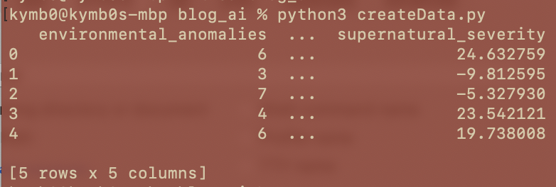
We will need the actual data (Bobby’s Field notes) to, well, exist. So we run the below script generate our dataset:

import pandas as pd
import numpy as np

np.random.seed(42)

environmental_anomalies = np.random.randint(0, 10, 100)
entity_signatures = np.random.randint(0, 5, 100)
sulfur_presence = np.random.randint(0, 3, 100)
angel_energy = np.random.normal(5.0, 1.5, 100)

supernatural_severity = (
    3.5 * environmental_anomalies +
    2.5 * entity_signatures +
    6.0 * sulfur_presence +
    -4.0 * angel_energy +
    np.random.normal(0, 5, 100)
)

data = pd.DataFrame({
    'environmental_anomalies': environmental_anomalies,
    'entity_signatures': entity_signatures,
    'sulfur_presence': sulfur_presence,
    'angel_energy': angel_energy,
    'supernatural_severity': supernatural_severity
})

data.to_csv('supernatural_dataset.csv', index=False)
print(data.head())

Training the Model

With the data now in existence, we need to load it into memory, label the variables as either input or output, and initialise the data model itself.

• Install JupyterLab
• pip install jupyterlab
• Then run with jupyter lab
• Start a new notebook with pykernel in the browser window that pops up
• Paste in and run the below

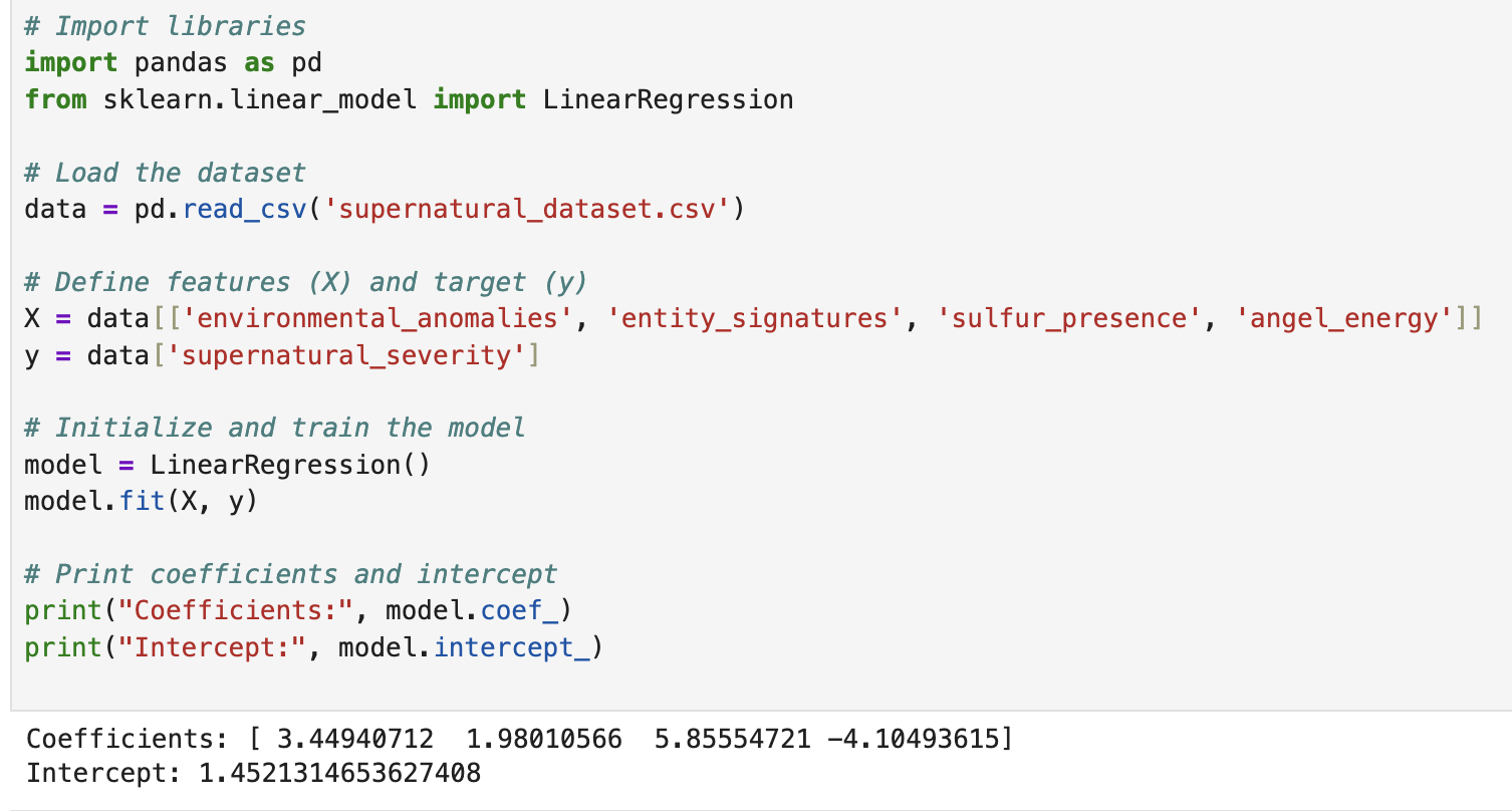
from sklearn.linear_model import LinearRegression

data = pd.read_csv('supernatural_dataset.csv')

X = data[['environmental_anomalies', 'entity_signatures', 'sulfur_presence', 'angel_energy']]
y = data['supernatural_severity']

model = LinearRegression()
model.fit(X, y)

print("Coefficients:", model.coef_)
print("Intercept:", model.intercept_)

What fit() Actually Does

When you call fit(X, y), you’re telling the model:

• Here are the inputs and their real outputs
• Learn the line that best maps inputs to outputs
• Do it by minimizing prediction error

Behind the scenes, this is OLS!!

• Guess some coefficients and an intercept
• Predict values using those guesses
• Compare to actual y, compute residuals
• Square the errors
• Adjust the numbers to reduce the total squared error
• Repeat until optimal

Visualizing Predictions

With the model now “trained” - we can visualise what we have done

import matplotlib.pyplot as plt

y_pred = model.predict(X)

plt.figure(figsize=(8,6))
plt.scatter(y, y_pred, color='blue', alpha=0.6, label='Predicted')
plt.plot([y.min(), y.max()], [y.min(), y.max()], color='red', linestyle='--', label='Perfect Fit')
plt.xlabel('Actual Supernatural Severity')
plt.ylabel('Predicted Supernatural Severity')
plt.title('Actual vs Predicted Severity')
plt.legend()
plt.grid(True)
plt.show()

• Each blue dot = a single event that was evaluated
• X-axis = the true supernatural severity (what actually happened)
• Y-axis = the model’s prediction (what was guessed to have happened)
• We see that the trend is strong in terms of most predictions closely following the known outcome (visualised by the dots tightly grouping the red line as it travels)

To see the residuals, we can further run the below:

# Calculate residuals (actual - predicted)
residuals = y - y_pred

# Plot residuals
plt.figure(figsize=(8,6))
plt.scatter(y_pred, residuals, alpha=0.6, color='purple')
plt.axhline(y=0, color='red', linestyle='--')
plt.xlabel('Predicted Supernatural Severity')
plt.ylabel('Residuals')
plt.title('Residuals vs Predicted Values')
plt.grid(True)
plt.show()

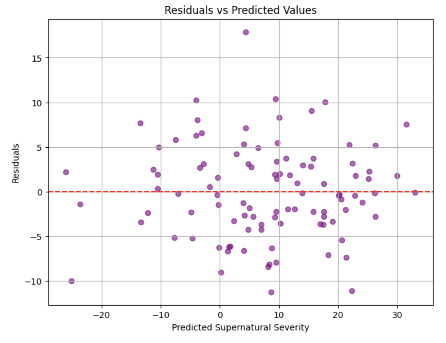
• Each purple dot = A single prediction
• X-axis = Y-axis = the model’s prediction (what was guessed to have happened)
• Y-axis = the value of actual - (minus) predicted - the residual aka how far off the model was for that prediction
• We see that the trend is strong in terms of residuals (errors) being scattered, if the residuals weren’t scattered, it would mean the model was consistently over or under-estimating in some regions

This chart is how you we would debug our model should we identify issues with predictions such as showing bias.

How Could This be Weaponised by an Adversary

The concept of weaponising input data is referred to as “Adversarial Machine Learning” - where someone with bad intentions has access to the inputs which in turn allows them to poison the model, and thus affect whatever occurs upstream as a result of any action taken by virtue of what the model predicts.

If we poison the data, we poison the prediction — and thus, poison the outcome

Example: A group of rival hunters or even a group of demon’s tasked with taking out Sam and Dean start visiting locations of sightings they will suspect Sam and Dean will respond to, and bring with them an Angel Blade to increase their sense of safety before ambushing them, or, deploy false evidence to mislead them into being ill-equipped to deal with whatever threat they would be facing.

WELCOME TO THE END

So that’s Linear Regression and OLS!!

Bobby is very proud of you for getting through this, and hopes to see you in the next installment.